Computational methods
Long reads
The Shasta assembler can be used to assemble DNA sequence fromn long reads. It is optimized especially for Oxford Nanopore reads, but can also be used to assemble other types of long reads such as those generated by Pacific Biosciences sequencing platforms.
Oxford Nanopore reads are rapidly evolving in characteristics, and therefore cannot be characterized precisely. Here is a summary of read metrics for the best available reads as of September 2020:
- Typical length around 50 Kb, with just a few percent of coverage in reads below 10 Kb and 10% or more of coverage in reads longer than 100 Kb. There are also Ultra-Long (UL) protocols that provide longer reads, with typical lengths around 100 Kb.
- Sequence identity around 97%, or equivalently an error rate around 3%. This relative high error rate has been improving significantly in time.
- The dominant error mode consists of errors in the length of homopolymer runs of all lengths. Errors in short homopolymer runs (lengths 1-5) are particularly deleterious due to their high frequency.
Computational challenges
Due to their length, Oxford Nanopore reads have unique value for de novo assembly. However a successful approach needs to deal with the high error rate.
Traditional approaches to de novo assembly typically rely on selecting a k-mer length that satisfies the following:
- K-mers of the selected length are reasonably unique in the target genome. For human assemblies, this typically means k ⪆ 30.
- Most k-mers of the selected length are error free in the target reads. This means that k must be significantly less than the inverse of the error rate.
For many sequencing technolgies the above conditions are satisfied for k around 30. But for our target reads, with an error rate around 3%, most 30-mers contains errors, and therefore assembly algorithms based on using such k-mers become unfeasible.
A possible approach consists of adding a preliminary error correction step in which reads are aligned to each other and corrected based on consensus, and then presenting to the assembler the corrected reads, which hopefully have a much lower error rate. But such approaches tends to be slow, and in addition any errors made in the error correction step are permanent and cannot be fixed during the assembly process.
Read representation
The computational techniques used in the Shasta assembler rely on representing the sequence of input reads in a way that the reduces the effect of errors on the de novo assembly process:
- The sequence of input reads is represented using run-length encoding.
- In many assembly steps, the sequence of input reads is described by using occurrences of a pre-determined subset of short k-mers (k ≈ 10 in run-encoding) called markers.
Run-length encoding
With run-length encoding, the sequence of each input read is represented as a sequence of bases, each with a repeat count that says how many times each of the bases is repeated. For example, the following read
CGATTTAAGTTAis represented as follows using run-length encoding:
CGATAGTA
11132121
Using run-length encoding makes the assembly process less sensitive to errors in the length of homopolymer runs, which are the most common type of errors in Oxford Nanopore reads. For example, consider these two reads:
CGATTTAAGTTA
CGATTAAGGGTTA
Using their raw representation above, these reads can aligned like this:
CGATTTAAG--TTA
CGATT-AAGGGTTA
Aligning the second read to the first required a deletion and two insertions. But in run-length encoding, the two reads become:
CGATAGTA
11132121
CGATAGTA
11122321
The sequence portions are now identical and can be aligned trivially and exactly, without any insertions or deletions:
CGATAGTA
CGATAGTA
The differences between the two reads only appear in the repeat counts:
11132121
11122321
   * *
The Shasta assembler uses one byte to represent repeat counts, and as a result it only represents repeat counts between 1 and 255. If a read contains more than 255 consecutive bases, it is discarded on input. Such reads are extremely rare, and the occurrence of such a large number of repeated bases is probably a symptom that something is wrong with the read anyway.
Some properties of base sequences in run-length encoding
- In the sequence portion of the run-length encoding, consecutive bases are always distinct. If they were not, the second one would be removed from the run-length encoded sequence, while increasing the repeat count for the first one.
- With ordinary base sequences, the number of distinct k-mers of length k is 4k. But with run-length base sequences, the number of distinct k-mers of length k is 4×3k-1. This is a consequence of the previous bullet.
- The run-length sequence is generally shorter than the raw sequence, and cannot be longer. For a long random sequence, the number of bases in the run-length representation is 3/4 of the number of bases in the raw representation.
Markers
Even with run-length encoding, error in input reads are still frequent. To further reduce sensitivity to errors, and also to speed up some of the computational steps in the assembly process, the Shasta assembler also uses a read representation based on markers. Markers are occurrences in reads of a pre-determined subset of short k-mers. By default, Shasta uses for this purpose k-mers with k=10 in run-length encoding, corresponding to an average approximately 13 bases in raw read representation.
Just for the purposes of illustration, consider a description using markers of length 3 in run-length encoding. There is a total 4×32 = 36 distinct such markers. We arbitrarily choose the following fixed subset of the 36, and we assign an id to each of the kmers in the subset:
TGC | 0 |
GCA | 1 |
GAC | 2 |
CGC | 3 |
Consider now the following portion of a read in run-length representation (here, the repeat counts are irrelevant and so they are omitted):
CGACACGTATGCGCACGCTGCGCTCTGCAGC
 GAC     TGC   CGC       TGC
           CGC    TGC     GCA
            GCA     CGC
Occurrences of the k-mers defined in the table above are shown
and define the markers in this read. Note that markers
can overlap. Using the marker ids defined in the table above,
we can summarize the sequence of this read portion as follows:
2 0 3 1 3 0 3 0 1This is the marker representation of the read portion above. It just includes the sequence of markers occurring in the read, not their positions.
In Shasta documentation and code, the zero-based sequence number of a marker in the marker representation of an oriented read is called the marker ordinal or simply ordinal. The first marker in an oriented read has ordinal 0, the second one has ordinal 1, and so on.
Note that the marker representation loses information, as it is not possible to reconstruct the complete initial sequence from the marker representation. This also means that the marker representation is insensitive to errors in the sequence portions that don't belong to any markers.
The Shasta assembler uses a random choice of the k-mers to be used
as markers. The length of the markers k is controlled by
assembly parameter
--Kmers.k
with a default value of 10.
Each k-mer is randomly choosen to be used as a marker
with probability determined by assembly parameter
--Kmers.probability
with a default value of 0.1.
With these default values, the total number of distinct
markers is approximately 0.1×410×39≈7900.
Options are also provided to read from a file the RLE k-mers to be used as markers. This permits experimentation with marker k-mers chosen in ways other than random. To date, no marker selection algorithm has proven more successful than random selection, but is is very possible that assembly quality can be improved by non-random selection of markers.
The only constraint used in selecting k-mers to be used as markers is that if a k-mer is a marker, its reverse complement should also be a marker. This makes it easy to construct the marker representation of the reverse complement of a read from the marker representation of the original read. It also ensures strand symetry in some of the computational steps.
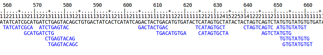
Below is the run-length representation of a portion of a read and its markers, as displayed by the Shasta http server.
Marker alignments
The marker representation is a sequence
The marker representation of a read is a sequence in an alphabet consisting of the marker ids. This sequence is much shorter than the original sequence of the read, but uses a much larger alphabet. For example, with default Shasta assembly parameters, the marker representation is 10 times shorter than the run-length encoded read sequence, or about 14 times shorter than the raw read sequence. Its alphabet has around 8000 symbols, many more than the 4 symbols that the original read sequence uses.Because the marker representation of a read is a sequence, we can compute an alignment of two reads directly in marker representation. Computing an alignment in this way has two important advantages:
- The shorter sequences and larger alphabet make the alignment much faster to compute.
- The alignment is insensitive to read errors in the portions that are not covered by any marker.
Alignment matrix
Consider two sequences on any alphabet, sequence x with nx symbols xi (i=0,...nx-1) and sequence y with ny symbols yj (j=0,...ny-1). The alignment matrix of the two sequences, , Aij, is a nx×ny matrix with elements
Aij = δxiyj
or, in words, Aij is 1 if xi=yj and 0 otherwise. (The Shasta assembler never explicitly constructs alignment matrices except for display when requested interactively. Alignment matrices are used here just for the purpose of illustration).
In portions where the sequences x and y are perfectly aligned, the alignment matrix consists of a matrix diagonal set to 1. Most of the remaining elements will be 0, but many can be 1 just because the same symbol appears at two unrelated locations in the two sequences.
Alignment matrix in raw base representation
The picture below shows a portion of a typical alignment matrix of two reads in their representation as a raw base sequence (not the run-length encoded representation) and a computed optimal alignment. This is for illustration only, as the Shasta assembler never constructs such a matrix, except when requested interactively.
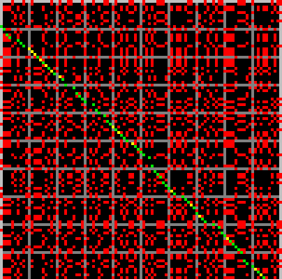
Here, elements of the alignment matrix are colored as follows:
- Red dots are alignment matrix elements that are 1 but that are not part of the computed optimal alignment.
- Green dots are alignment matrix elements that are 1 and that are part of the computed optimal alignment.
- Yellow matrix elements are alignment matrix elements that are 0 but that were computed to be part of the optimal alignment as mismatching alignment positions.
- Black or grey matrix elements are matrix elements that are 0 and that were not computed to be part of the optimal alignment. Grey is used instead of black every 10 bases to facilitate counting bases in the figure.
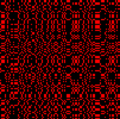
On average, about 25% of the matrix elements are 1, simply because the alphabet has 4 symbols. Because of the large fraction of 1 elements and because of the high error rate, it would be hard to visually locate the optimal alignment in this picture, if it was not highlighted using colors. This is emphasized by the following figure, which represents the same matrix, but with all 1 elements now colored red and all 0 elements black.
Note that the alignment matrix contains frequent square or rectangular blocks of 1 elements. They correspond to homopolymer run. A square block indicates that the two reads agree on the length of that homopolymer run, and a non-square rectangular block indicates that the two reads disagree. If we were using run-length encoding for this picture, these blocks would all collapse to a single matrix element.
Alignment matrix in marker representation
For comparison, the picture below shows a portion of the alignment matrix of two reads, in marker representation, as displayed by the Shasta http server. In this alignment matrix, the marker ordinal on the first read is on the horizontal axis (increasing towards the right) and the marker ordinal for the second read (increasing towards the bottom) is on the vertical axis. Here, matrix elements that are 1 are displayed in green or red. The ones in green are the ones that are part of the optimal alignment computed by the Shasta assembler - see below for more information. The grey lines are drawn 10 markers apart from each other and their only purpose is to facilitate reading the picture - the corresponding matrix elements are 0. Shasta marker alignments only include matching markers and gaps. Mismatching markers are never included in the alignment.
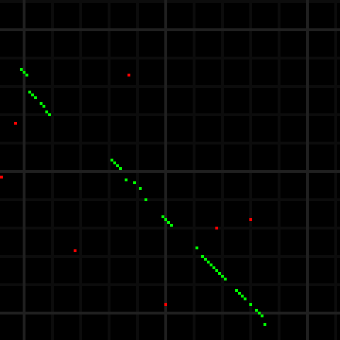
Because of the much larger alphabet, matrix elements that are 1 but are not part of the optimal alignment are infrequent. In addition, each alignment matrix element here corresponds on average to a 13×13 block in the alignment matrix in raw base sequence shown above. The portion of alignment matrix in marker space shown here covers about 120 markers or about 1500 bases in the original representation of the read, compared to only about 100 bases in the alignment matrix in raw representation shown above . For these reasons, the marker representation is orders of magnitude more efficient than the raw base representation when computing read alignments.
Alignment metrics
Shasta uses several metrics to characterize alignments in marker space. As shown in the picture above, a typical alignment consists of stretches of consecutive aligned markers intermixed with gaps in the alignment. Call xi (i=0,...,N-1) the aligned marker ordinals on the first oriented read and yj (j=0,...,N-1) the aligned marker ordinals on the second oriented read, where N is the number of aligned markers. That is, xi and yi are the coordinates of the green points in the alignment matrix as depicted above. Also call Nx the number of markers in the first oriented read and Ny the number of markers in the second oriented read. Nx and Ny are the horizontal and vertical sizes, respectively, of the alignment matrix.
With this notation, we define the following metrics for a marker alignment. For each metric, there is a command line option that controls the minimum or maximum value of the metric for an alignment to be considered valid and used in the assembly. These options can be used to control the quality of marker alignments to be used during assembly.
- N
is the number of aligned markers.
An alignment is only used if N
is at least equal to the value of
--Align.minAlignedMarkerCount. This option can be used to discard alignments that are too short to be considered reliable. -
For each oriented read in the alignment, the
alignedFractionis defined as the ratio of the number of aligned markers over the length of the range of ordinals covered by the alignment, that is N / (xN-1 - x0 + 1) for the first oriented read and N / (yN-1 - y0 + 1) for the second oriented read. The lesser of thealignedFractionof the two oriented reads is called thealignedFractionof the alignment. It is a measure of the accuracy of the alignment. An alignment is only used ifalignedFraction is at least equal to the value of --Align.minAlignedFraction.- The maximum number of markers skipped by any alignment gap (on either ot the two oriented reads) is called
skipand is defined as the maximum value of max(xi+1 - xi, yi+1 - yi) computed over i=1,...,N-1. Note that, with this definition, gaps at the beginning and end of the alignment are not considered (but seetrimbelow). An alignment is only used ifskipis at most equal to the value of--Align.maxSkip. This option can be used to discard alignments containing long gaps.- Even when an alignment gap occurs, successive aligned markers tend to be approximately on the same diagonal of the alignment matrix. This reflects the fact that, even when sequencing errors occur, the number of bases read is likely to still be approximately correct. The maximum diagonal shift between successive aligned markers is called
driftand is defined as the maximum value of the absolute value of (xi+1 - yi+1) - (xi - yi) computed over i=1,...,N-1. Note that, in this case too, alignment gaps at the beginning and end of the alignment are not considered. An alignment is only used ifdriftis at most equal to the value of--Align.maxDrift. This option can be used to discard alignments containing gaps with large diagonal shift.- An alignment should always begins near the beginning of at least one of the two oriented reads, but we need to allow for an initial incorrect portion at the beginning of each read. The minimum over the two oriented reads of the number of markers skipped at the beginning of the alignment, min(x0, y0) is called the
leftTrim. Similarly, the minimum over the two oriented reads of the number of markers skipped at the end of the alignment, min(Nx - 1 - xN-1, Ny - 1 - yN-1) is called therightTrim. The lesser ofleftTrimandrightTrimis calledtrimAn alignment is only used iftrim. is at most equal to the value of--Align.maxTrim. - The maximum number of markers skipped by any alignment gap (on either ot the two oriented reads) is called
Computing optimal alignments in marker representation
To compute the optimal alignment highlighted in green in the above figure,
one of the folowing methods is used,
under control of command line option
--Align.alignMethod:
--Align.alignMethod 0selects the legacy Shasta algorithm. Do not use for production assemblies.--Align.alignMethod 1computes marker alignments using SeqAn. Do not use for production assemblies.--Align.alignMethod 3(the default choice) uses a faster two-step algorithm that also uses SeqAn and achieves better performance using a combination of downsampling and banded alignments.
The computation of marker alignments for all alignment candidates
found by the
LowHash algorithm
is one of the most expensive
phases of an assembly, and typically takes around half of
total elapsed time.
For this reason, it is recommended that only
the default --Align.alignMethod 3
be used for production assemblies.
--Align.alignMethod 0
This selects
a simple alignment algorithm
on the marker representations of the two reads to be aligned.
Do not use this method for production assemblies,
as the default alignment method selected by
--Align.alignMethod 3
provides better performance and accuracy.
This algorithm effectively constructs an optimal path in the alignment matrix,
but using some heuristics to speed up the computation:
- The maximum number of markers that an alignment
can skip on either read is limited to a maximum,
under control of assembly parameter
--Align.maxSkip(default value 30 markers, corresponding to around 400 bases when all other Shasta parameters are at their default). This reflects the fact that Oxford Nanopore reads can often have long stretches in error. In the alignment matrix shown above, there is a skip of about 20 markers (2 light grey squares) following the first 10 aligned markers (green dots) on the top left. - The maximum number of markers that an alignment
can skip at the beginning or end of a read is limited to a maximum,
under control of assembly parameter
--Align.maxTrim(default value 30 markers, corresponding to around 400 bases when all other Shasta parameters are at their default). This reflects the fact that Oxford Nanopore reads often have an initial or final portion that is not usable. - To avoid alignment artifacts,
marker k-mers that are too frequent in either of the two reads
being aligned are not used in the alignment computation.
For this purpose, the Shasta assembler uses a criterion based
on absolute number of occurrences of marker k-mers in the two reads,
although a relative criterion (occurrences per Kb) may be more appropriate.
The current absolute frequency threshold is under control of assembly parameter
--Align.maxMarkerFrequency(default 10 occurrences).
--Align.alignMethod 1
This causes marker alignments to be computed using
SeqAn overlap alignments.
This guarantees an optimal alignment, but is computationally very expensive,
with cost proportional to the size of the alignment matrix,
therefore O(N2) in the number of markers
in the two reads being aligned.
Do not use this method for production assemblies,
as the default alignment method selected by
--Align.alignMethod 3 provides much better performance
with minimal degradation in accuracy.
--Align.alignMethod 3
This is the default alignment method used by Shasta and provides a good combination of performance and accuracy. It uses the SeqAn in a two-step process:
- In a first step, SeqAn is used to compute an overlap alignment between two downsampled versions of the marker sequences of the reads to be aligned. This is O(N2) in the number of markers in the two reads being aligned, but still reasonably fast because od downsampling.
- In a second step, SeqAn is used to compute a banded alignment of the markerrepresentation of the two reads. The position and width of the band is obtained from the downsampled alignment computed in the first step.
Finding overlapping reads
Even though computing read alignments in marker representation is fast, it still is not feasible to compute alignments among all possible pairs of reads. For a human size genome with ≈106-107 reads, the number of pairs to consider would be ≈1012-1014, and even at 10-3 seconds per alignment the compute time would be ≈109-1011 seconds, or ≈107-109 seconds elapsed time (≈102-104 days) when using 128 virtual processors.
Therefore some means of narrowing down substantially the number of pairs to be considered is essential. The Shasta assembler uses for this purpose a slightly modified MinHash scheme based on the marker representation of reads.
For a general description of the MinHash algorithm see the Wikipedia article or this excellent book chapter. In summary, the MinHash algorithm takes as input a set of items each characterized by a set of features. Its goal is to find pairs of the input items that have a high Jaccard similarity index - that is, pairs of items that have many features in common. The algorithm proceeds by iterations. At each iteration, a new hash table is created and a hash function that operates on the feature set is selected. For each item, the hash function of each of its features is evaluated, and the minimum hash function value found is used to select the hash table bucket that each item is stored in. It can be proven that the probability of two items ending up in the same bucket equals the Jaccard similarity index of the two items - that is, items in the same bucket are more likely to be highly similar than items in different buckets. The algorithm then adds to the pairs of potentially similar items all pairs of items that are in the same bucket.
When all iterations are complete, the probability that a pair of items was found at least once is an increasing function of the Jaccard similarity of the two items. In other words, the pairs found are enriched for pairs that have high similarity. One can now consider all the pairs found (hopefully a much smaller set than all possible pairs) and compute the Jaccard similarity index for each, then keep only the pairs for which the index is sufficiently high. The algorithm does not guarantee that all pairs with high similarity will be found - only that the probability of finding all pairs is an increasing function of their similarity.
The algorithm is used by Shasta with items being oriented reads (a read in either original or reverse complemented orientation) and features being consecutive occurrences of m markers in the marker representation of the oriented read. For example, consider an oriented read with the following marker representation:
18,45,71,3,15,6,21If m is selected equal to 4 (the Shasta default, controlled by assembly parameter
--MinHash.m),
the oriented read is assigned the following features:
(18,45,71,3)
(45,71,3,15)
(71,3,15,6)
(3,15,6,21)
From the picture above of an alignment matrix in marker representation, we see that streaks of 4 or more common consecutive markers are relatively common. We have to keep in mind that, with Shasta default parameters, 4 consecutive markers span an average 40 bases in run-length encoding or about 52 bases in the original raw base representation. At a typical error rate around 10%, such a portion of a read would contain on average 5 errors. Yet, the marker representation in run-length space is sufficiently robust that these common "features" are relatively common despite the high error rate. This indicates that we can expect the MinHash algorith to be effective in finding pairs of overlapping reads.
However, the MinHash algorithm has a feature that is undesirable for our purposes: namely, that the algorithm is good at finding read pairs with high Jaccard similarity index. For two sets X and Y, the Jaccard similarity index is defined as the ratio
J = |X∩Y| / |X∪Y|Because the read length distribution of Oxford Nanopore reads is very wide, it is very common to have pairs of reads with very different lengths. Consider now two reads with lengths nx and ny, with nx<ny, that overlap exactly over the entire length nx. The Jaccard similarity is in this case given by nx/ny < 1. This means that, if one of the reads in a pair is much shorter than the other one, their Jaccard similarity will be low even in the best case of exact overlap. As a result, the unmodified MinHash algorithm will not do a good job at finding overlapping pairs of reads with very different length.
For this reason, the Shasta assembler uses a small modification to the MinHash algorithm: instead of just using the minimum hash for each oriented read for each iteration, it keeps all hashes below a given threshold. Each oriented read can be stored in multiple buckets, one for each low hash encountered. This has the effect of eliminating the bias against pairs in which one read is much shorter than the other. The modified algorithm is referred to as LowHash in the Shasta source code. It is effectively equivalent to a an indexing approach in which we index all features with low hash.
The LowHash algorithm is controlled by the following assembly parameters:
-
--MinHash.m(default 4): the number of consecutive markers that define a feature. -
--MinHash.hashFraction(default 0.01): The fraction of hash values that count as "low". -
--MinHash.minHashIterationCount(default 10): The number of iterations. -
--MinHash.maxBucketSize(default 10): The maximum number of items for a bucket to be considered. Buckets with more than this number of items are ignored. The goal of this parameter is to mitigate the effect of common repeats, which can result in buckets containing large numbers of unrelated oriented reads. -
--MinHash.minBucketSize(default 0): The minimum number of items for a bucket to be considered. Buckets with less than this number of items are ignored, because MinHash features in these buckets are likely to be in error. -
--MinHash.minFrequency(default 2): the number of times a pair of oriented reads has to be found to be considered and stored as a possible pair of overlapping reads.
Initial assembly steps
Initial steps of a Shasta assembly proceed as follows.
If the assembly is setup for
best performance
(--memoryMode filesystem --memoryBacking 2M
if using the Shasta executable), all data structures
are stored in memory, and no disk activity takes
place except for initial loading of the input reads,
storing of assembly results, and storing a small number
of small files with useful summary information.
- Input reads are read from Fasta files and converted
to run-length representation. Read shorter
than the read length cutoff
--Reads.minReadLengthbases (default 10000) are discarded. Reads that contain bases with repeat counts greater than 255 are also discarded. This is a consequence of the fact that repeat counts are stored using one byte, and therefore there would be no way to store such reads. Reads with such long repeat counts are extremely rare, however, and when they occur they are of suspicious quality. - In addition, if a non-zero value is specified for
--Reads.desiredCoverage, the read length cutoff is further increased until coverage is just above the specified number of bases. - K-mers to be used as markers are randomly selected.
- Occurrences of those marker k-mers in all oriented reads are found.
- The LowHash algorithm finds candidate pairs of overlapping oriented reads.
- A marker alignment is computed for each candidate pair of oriented reads. If the alignment metrics are sufficiently good, the alignment is stored for use in the assembly.
Read graph
Using the methods covered so far, an assembly has created a list of pairs of oriented reads, each pair having a plausible marker alignment. How to use this type of information for assembly is a classical problem with a standard solution (Myers, 2005), the string graph. However, the prescriptions in the Myers paper cannot be directly used here, mostly due to the marker representation.
Shasta proceeds by creating a Read Graph, an undirected
graph in which each vertex corresponds to an oriented read.
A subset of the available alignments is selected using one of two
methods described below, under control of command line option
--ReadGraph.creationMethod.
For each selected alignment, an undirected edge is created in the read
graph between the vertices corresponding to the oriented reads
in the selected alignment.
If we used all of the available alignments to create read graph edges, the resulting read graph would suffers from high connectivity in repeat regions, due to spurious alignments between oriented reads originating in different but similar regions of the genome. Therefore it is important to select alignments to be used in a way that minimizes these spurious alignments while keeping true ones as much as possible.
Note that each read contributes two vertices to the read graph, one in its original orientation, and one in reverse complemented orientation. Therefore the read graph contains two strands, each strand at full coverage. This makes it easy to investigate and potentially detect erroneous strand jumps that would be much less obvious if using alternative approaches with one vertex per read.
An example of a portion of the read graph, as displayed
by the Shasta http server, is shown here.
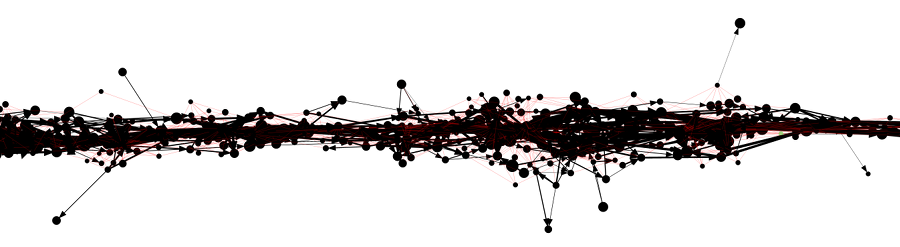
Even though the graph is undirected, edges that correspond to overlap alignments are drawn with an arrow that points from the leftmost oriented read to the rightmost one. Edges that correspond to containment alignments are drawn in red and without an arrow. Vertices are drawn with area proportional to the length of the corresponding reads.
The linear structure of the read graph successfully reflects the linear arrangement of the input reads and their origin on the genome being assembled.
However, deviations from the linear structure can
occur in the presence of long repeats,
typically for high similarity segment duplications:
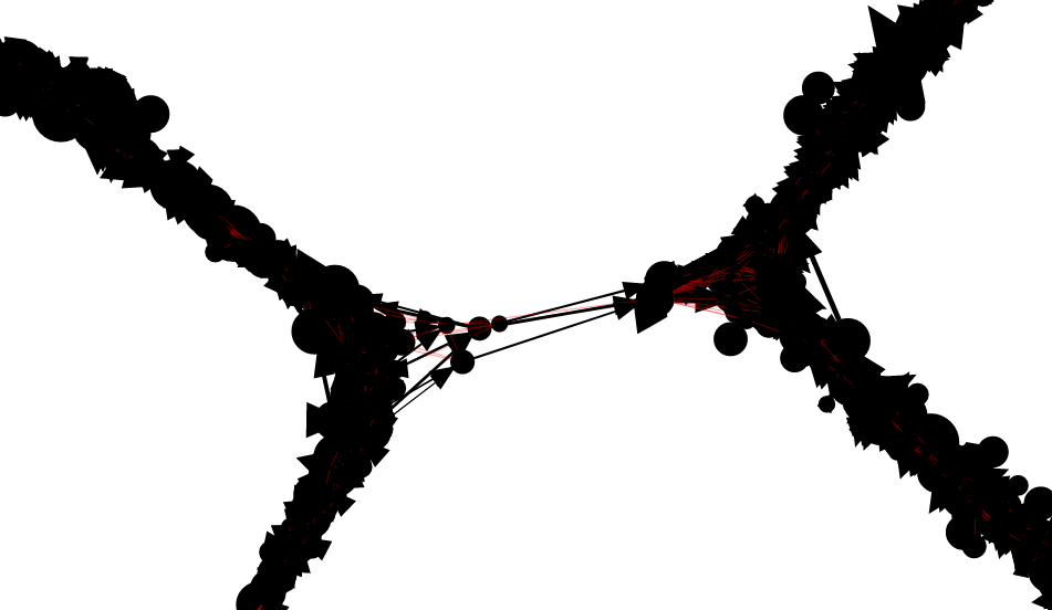
The obviously incorrect connections can destroy the linear structure of assembled sequence. This is dealt with later in the assembly process.
Read graph creation method 0
When --ReadGraph.creationMethod 0
(the default) is selected, the Shasta assembler uses a very simple method to select
alignments: it only keeps a
k-Nearest-Neighbor
subset of the alignments.
That is, for each vertex (oriented read)
it only keeps the best k alignments,
as measured by the number of aligned markers.
The number of edges k kept
for each vertex is controlled by assembly option
--ReadGraph.maxAlignmentCount,
with a default value of 6.
Note that, despite the k-Nearest-Neighbor subset,
it remains possible for a vertex to have degree
more than k.
Read graph creation method 2
When --ReadGraph.creationMethod 2
is selected, a more sophisticated approach,
developed by Ryan Lorig-Roach at U. C. Santa Cruz,
is used.
Shasta first inspects all stored alignments to compute
statistical distributions (histograms) for the five alignment
metrics in the table below.
Alignments for which one of these metrics is worse than a set percentile
are discarded. The threshold percentiles are controlled by
the command line options shown in the table.
| Alignment metric | Percentile option | Default value |
|---|---|---|
| Number of aligned markers | --ReadGraph.markerCountPercentile
| 0.015 |
| Aligned marker fraction | --ReadGraph.alignedFractionPercentile
| 0.12 |
| Maximum number of markers skipped | --ReadGraph.maxSkipPercentile
| 0.12 |
| Maximum diagonal drift | --ReadGraph.maxDriftPercentile
| 0.12 |
| Number of markers trimmed | --ReadGraph.maxTrimPercentile
| 0.015 |
The process than continues with the same
k-Nearest-Neighbor procedure used with
--ReadGraph.creationMethod 0,
but only considering alignments that were not ruled
out by above percentile criteria.
Because of its adaptiveness to alignment characteristics,
this method is more robust and less sensitive
to the choice of alignment criteria,
and results in more accurate and more contiguous assemblies.
However, when using --ReadGraph.creationMethod 2
it is important to use very liberal choices for the
options that control alignment quality, because
bad alignments will be discarded anyway using the
percentile criteria.
An example of assembly options with --ReadGraph.creationMethod 2
is provided in Shasta configuration files
Nanopore-Sep2020.conf and
Nanopore-UL.Sep2020.conf.
These files apply to Oxford Nanopore reads created
with base caller Guppy version 3.6.0 or newer
(standard and ultra-long version, respectively).
They are available in the
conf directory in the source code tree
or in a Shasta build.
Marker graph
Consider a read whose marker representation is:
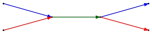
a b c d eWe can represent this read as a directed graph that the describes the sequence in which its markers appear:
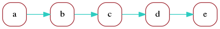
This is not very useful but illustrates the simplest form of a marker graph as used in the Shasta assembler. The marker graph is a directed graph in which each vertex represents a marker and each edge represents the transition between consecutive markers. We can associate sequence with each vertex and edge of the marker graph:
- Each vertex is associated with the sequence of the corrersponding marker.
- If the markers of the source and target vertex of an edge do not overlap, the edge is associated with the sequence intervening between the two markers.
- If the markers of the source and target vertex of an edge do overlap, the edge is associated with the overlapping portion of the marker sequences.
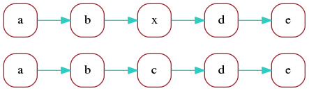
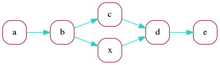
Consider now a second read with the following marker
representation, which differs from the previous one
just by replacing marker c with x:
a b x d e
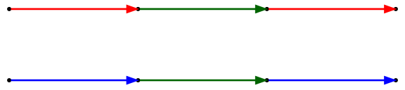
The marker graph for the two reads is:
In the optimal alignment of the two reads, markers
a, b, d, e are aligned. We can redraw the marker graph
grouping together vertices that correspond to aligned markers:
Finally, we can merge aligned vertices to obtain a marker graph describing the two aligned reads:
Here, by construction each vertex still has a unique
sequence associated with it - the common sequence
of the markers that were merged
(however the corresponding repeat counts
can be different for each contributing read).
An edge, on the other hand, can have different sequences
associated with it, one corresponding to each
of the contributing reads.
In this example, edges a->b
and d->e have two contributing reads,
which can each have distinct sequence between
the two markers.
We call coverage of a vertex or edge the number of reads "contributing"
to it. In this example, vertices a, b, d, e have coverage 2
and vertices c, x have coverage 1.
Edges a->b
and d->e have coverage 2, and the remaining edges have coverage 1.
The construction of the marker graph was illustrated above for two reads, but the Shasta assembler constructs a global marker graph which takes into account all oriented reads:
- The process starts with a distinct vertex for each marker of each oriented read. Note that at this stage the marker graph is large (≈ 2×10¹⁰ vertices for a human assembly using default assembly parameters).
- For each marker alignment corresponding to an edge of the read graph, we merge vertices corresponding to aligned markers.
- Of the resulting merged vertices, we remove those whose
coverage in too low or two high, indicating that the contributing
reads or some of the alignments involved are probably in error.
This is controlled by assembly parameters
MarkerGraph.minCoverage(default 10) andMarkerGraph.maxCoverage(default 100), which specify the minimum and maximum coverage for a vertex to be kept. - Edges are created. An edge
v0->v1is created if there is at least a read contributing to bothv0andv1and for which all markers intervening betweenv0andv1belong to vertices that were removed.
Given the large number of initial vertices involved, this computation is not trivial. To allow efficient computation in parallel on many threads, a lock-free implementation of the disjoint data set data structure, as first described by Anderson and Woll (1991), Anderson and Woll (1994), is used for merging vertices. Some code changes were necessary to permit large numbers of vertices, as the initial implementation by Wenzel Jakob only allowed for 32-bit vertex ids.
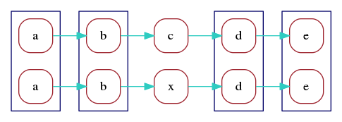
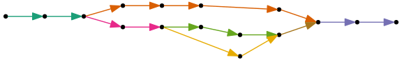
A portion of the marker graph, as displayed by the Shasta http server, is shown here:
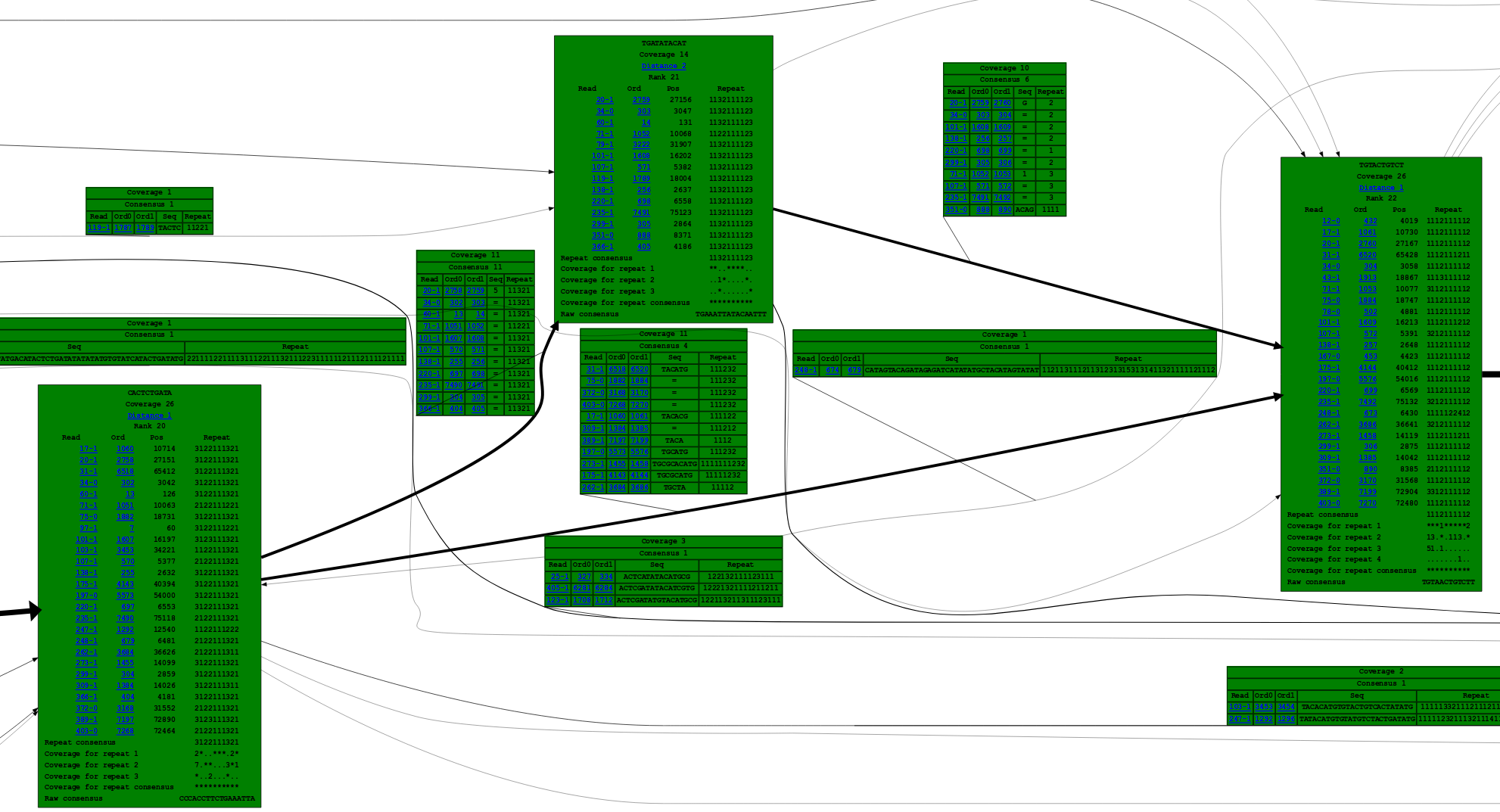
Each vertex, shown in green, contains a list of the oriented reads the contribute to it. Each oriented read is labeled with the read id (a number) followed by "-0" for original orientation and "-1" for reverse complemented orientation. Each vertex is also labeled with the marker sequence (run-length encoded). Edges are drawn with an arrow whose thickness is proportional to edge coverage, and labeled with the sequence contributed by each read. In edge labels, a sequence consisting of a number indicates the number of overlapping bases between adjacent markers.
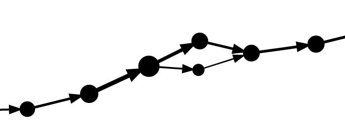
On as larger scale and with less detail, a typical portion of the marker graph looks like this:
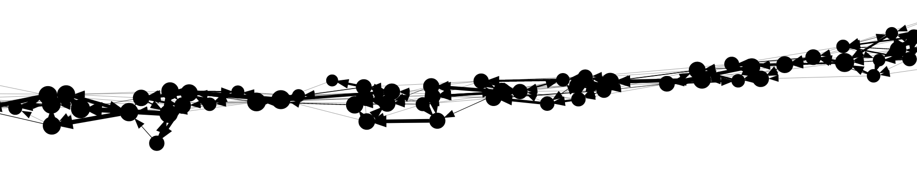
Here, each vertex is drawn with size proportional to its coverage. Edge arrows are again displayed with thickness porportional to edge coverage. The marker graph has a linear structure with a dominant path and side branches due to errors.
Assembly graph
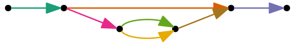
The Shasta assembly process also uses a compact representation of the marker graph, called the assembly graph, in which each linear sequence of edges is replaced by a single edge. For example, this marker graph
can be represented as an assembly graph as follows. Colors were chosen to indicate the correspondance to marker graph edges:
The length of an edge of the assembly graph is defined as the number of marker graph edges that it corresponds to. For each edge of the assembly graph, an average coverage is also computed, by averaging the coverage of the marker graph edges it corresponds to.
Using the marker graph to assemble sequence
The marker graph is a partial description of the multiple sequence alignment between reads and can be used to assemble consensus sequence. One simple way to do that is to only keep the "dominant" path in the graph, and then move on that path from vertex to edge to vertex, assembling run-length encoded sequence as follows:
- On a vertex, all reads have the same sequence, by construction: the marker sequence associated with the vertex. There is trivial consensus among all the reads contributing to a vertex, and the marker sequence can be used directly as the contribution of the vertex to assembled sequence.
- For edges, there are two possible situations plus a hybrid case:
- 2.1. If the adjacent markers overlap, in most cases all contributing reads have the same number of overlapping bases between the two markers, and we are again in a situation of trivial consensus, where all reads contribute the same sequence, which also agrees with the sequence of adjacent vertices. In cases where not all reads are in agreement on the number of overlapping bases, only reads with the most frequent number of overlapping bases are taken into account.
- 2.2. If the adjacent markers don't overlap, then each read can have a different sequence between the two markers. In this situation, we compute a multiple sequence alignment of the sequences and a consensus using the Spoa library. The multiple sequence alignment is computed constrained at both ends, because all reads contributing to the edge have, by construction, identical markers at both sides.
- 2.3. A hybrid situation occasionally arises, in which some reads have the two markers overlapping, and some do not. In this case we count reads of the two kinds and discard the reads of the minority kind, then revert to one of the two cases 2.1 or 2.2 above.
This is the process used for sequence assembly by the current Shasta implementation. It requires a process to select and define dominant paths, which is described in the next section. It is algorithmically simple, but its main shortcoming is that it does not use for assembly reads that contribute to the abundant side branches. This means that coverage is lost, and therefore the sequence of assembled accuracy is not as good as it could be if all available coverage was used. Means to eliminate this shortcoming and use information from the side branches of the marker graph could be a subject of future work on the Shasta assembler.
Assembling repeat counts
The process described above works with run-length encoded sequence and therefore assembles run-length encoded sequence. The final step to create raw assembled sequence is to compute the most likely repeat count for each sequence position in run-length encoding. In Shasta 0.1.0 this was done done by choosing as the most likely repeat count the one that appears the most frequently in the reads that contributed to each assembled position.
The latest version of the Shasta assembler supports three different options
for that, under control of command line option
--Assembly.consensusCaller:
--Assembly.consensusCaller Modalrequests the same algorithm used in Shasta 0.1.0, that is, the most frequent repeat count seen at each base position is used in the assembly.--Assembly.consensusCaller Medianrequests an algorithm that stores in the assembly the median repeat count seen at each base position.--Assembly.consensusCaller Bayesian:namerequests a Bayesian algorithm to determine the most likely repeat count.namecan be one of the following:- One of the following built-in Bayesian models:
guppy-2.3.1-ato use a Bayesian model optimized for the Guppy 2.3.1 base caller.guppy-2.3.5-a(the default) to use a Bayesian model optimized for the Guppy 2.3.5 base caller.guppy-3.0.5-ato use a Bayesian model optimized for the Guppy 3.0.5 base caller.guppy-3.4.4-ato use a Bayesian model optimized for the Guppy 3.4.4 base caller.guppy-3.6.0-ato use a Bayesian model optimized for the Guppy 3.6.5 base caller.r10-guppy-3.4.8-ato use a Bayesian model optimized for r10 reads and the Guppy 3.4.8 base caller.
- The name of a configuration file
describing the Bayesian model to be used,
which can be specified as a relative or absolute path.
Earlier versions of Shasta required an absolute path, but this
is no longer the case.
Sample configuration files are available in
shasta/conforshasta-install/conf. They are namedSimpleBayesianConsensusCaller-*.csv.
- One of the following built-in Bayesian models:
--Assembly.consensusCaller Bayesian:guppy-2.3.5-a.
Some testing showed a significant decrease of false positive indels
in assembled sequence compared to Shasta 0.1.0 behavior, corresponding to
--Assembly.consensusCaller Modal. This testing was done
for reads called using Guppy 2.3.5. However even using
--Assembly.consensusCaller Bayesian:guppy-2.3.1-a
resulted in significant improvement over
--Assembly.consensusCaller Modal, indicating
that the Bayesian model is somewhat resilient to
discrepancies between the reads used to construct the Bayesian model
and the reads being assembled.
Testing also showed that
--Assembly.consensusCaller Median is generally inferior to
--Assembly.consensusCaller Modal.
Selecting assembly paths
The sequence assembly procedure described in the previous section
can be used to assemble sequence for any path in the marker graph.
This section describes the selection of paths for assembly
in the current Shasta implementation.
This is done by a series of steps that "remove" edges
(but not vertices) from the marker graph until the
marker graph consists mainly of linear sections
which can be used as the assembly paths.
For speed, edges are not actualy removed but just marked
as removed using a set of flag bits allocated for this
purpose in each edge.
However, the description below will use the loose term remove
to indicate that an edge was flagged as removed.
This process consists of the following three steps, described in more detail in the following sections:
- Approximate transitive reduction of the marker graph.
- Pruning of short side branches (leaves).
- Removal of bubbles and super-bubbles.
Approximate transitive reduction of the marker graph
The goal of this step is to eliminate the side branches in the marker
graph, which are the result of errors.
Despite the fact that
the number of side branches is substantially reduced thanks to the use of
run-length encoding, side branches are still abundant.
This step uses an approximate transitive reduction of the marker graph which only
considers reachability up to a maximum distance,
controlled by assembly parameter
MarkerGraph.maxDistance
(default 30 marker graph edges).
Using a maximum distance makes sure that the process remains computationally affordable,
and also has the advantage of not removing long-range edges in the marker graph,
which could be significant.
In detail, the process works as follows.
In this description, the edge being considered for removal
is the edge v0→v1 with source vertex v0
and target vertex v1.
The first two steps are not really part of the transitive reduction
but are performed by the same code for convenience.
- All edges with coverage less than or equal to
MarkerGraph.lowCoverageThresholdare unconditionally removed. The default value for this assembly parameter is 0, so this step does nothing when using default parameters. - All edges with coverage 1
and for which the only supporting read has a large marker skip
are unconditionally removed.
The marker skip of an edge, for a given read, is defined as the distance
(in markers) between the
v0marker for that read and thev1marker for the same read. Most marker skips are small, and a large skip is indicative of an artifact. Keeping those edges could result in assembly errors. The marker skip threshold is controlled by assembly parameterMarkerGraph.edgeMarkerSkipThreshold(default 100 markers). - Edges
with coverage greater than
MarkerGraph.lowCoverageThreshold(default 0) and less thanMarkerGraph.highCoverageThreshold(default 256), and that were not previously removed, are processed in order of increasing coverage. Note that with the default values of these parameters all edges are processed, because edge coverage is stored using one byte and therefore can never be more than 255 (it is saturated at 255). For each edgev0→v1, a Breadth-First Search (BFS) in the marker graph is performed starting at source vertexv0and with a limit ofMarkerGraph.maxDistance(default 30) edges distance from vertexv0. The BFS is constrained to not use edgev0→v1. If the BFS reachesv1, indicating that an alternative path fromv0tov1exists, edgev0→v1is removed. Note that the BFS does not use edges that have already been removed, and so the process is guaranteed not to affect reachability. Processing edges in order of increasing coverage makes sure that low coverage edges are more the most likely to be removed.
When the transitive reduction step is complete, the marker graph consists mostly of linear sections composed of vertices with in-degree and out-degree one, with occasional side branches and bubbles or superbubbles, which are handled in the next two phases described below.
Pruning of short side branches (leaves)
At this stage, a few iterations of pruning are done
by simply removing, at each iteration,
edge v0→v1 if
v0 has in-degree 0 (that is, is a backward-pointing leaf)
or v1 has out-degree 0 (that is, is a forward-pointing leaf).
The net effect is that all side branches of length
(number of edges)
at most equal to the number of iterations are removed.
This leaves the leaf vertex isolated, which causes no problems.
The number of iterations is controlled
by assembly parameter
MarkerGraph.pruneIterationCount
(default 6).
Removal of bubbles and superbubbles
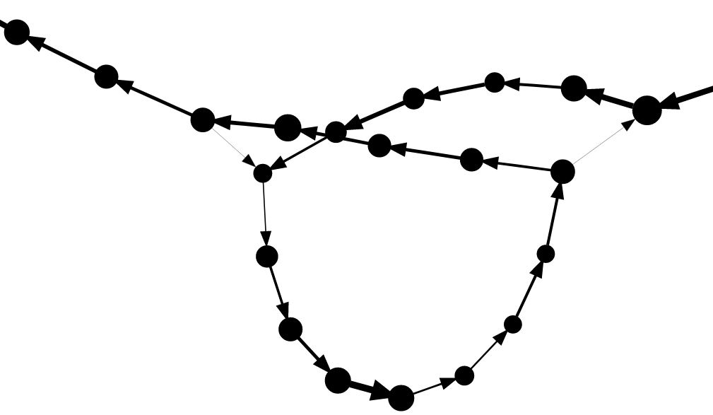
The marker graph now consists of mostly linear section with occasional bubbles or superbubbles. Most of the bubbles and superbubbles are caused by errors, but some of those are due to heterozygous loci in the genome being assembled. Bubbles and superbubbles of the latter type could be used for separating haplotypes (phasing) - a possibility that will be addressed in future Shasta releases. However, the goal of the current Shasta implementation is to create a haploid assembly at all scales but the very long ones. Accordingly, bubbles and superbubbles at short scales are treated as errors, and the goal of the bubble/superbubble removal step is to keep the most significant path in each bubble or superbubble.
The figures below show typical examples of a bubble and superbubble in the marker graph.
The bubble/superbubble removal process is iterative.
Early iterations work on short scales, and late iterations
fork on longer scales.
Each iteration uses a length threshold
that controls the maximum number of marker graph edges for
features to be considered for removal.
The value of the threshold for each iteration
is specified using assembly parameter
MarkerGraph.simplifyMaxLength,
which consists of a comma-separated string of integer
numbers, each specifying the threshold for one iteration
in the process. The default value is
10,100,1000, which means that three iterations
of this process are performed.
The first iteration uses a threshold of 10 marker graph edges,
and the second and third iterations
use length thresholds of 100 and 1000 marker graph edges, respectively.
The last and largest of the threshold values used
determines the size of the smallest bubble or superbubble
that will survive the process.
The default 1000 markers is equivalent to roughly 13 Kb.
To suppress more bubble/superbubbles, increase
the threshold for the last iterarion.
To see more bubbles/superbubbles, decrease
the length threshold for the last iteration, or remove the last iteration entirely.
The goal of the increasing threshold values is to work
on small features at first, and on larger features in the later iterations.
The best choice of
MarkerGraph.simplifyMaxLength
is application dependent. The default value
is a reasonable compromise useful if one desires
a mostly haploid assembly with just some large heterozygous features.
Each iteration consists of two steps. The first removes bubbles and the second removes superbubbles. Only bubbles/superbubbles consisting of features shorter than the threshold for the current iteration are considered:
- Bubble removal
- An assembly graph corresponding to the current marker graph is created.
- Bubbles are located in which the length of all branches (number of marker graph edges) is no more than the length threshold at the current iteration. In the assembly graph, a bubble appears as a set of parallel edges (edges with the same source and target).
- In each bubble, only the assembly graph edge with the highest average coverage is kept. Marker graph edges corresponding to all other assembly graph edges in the bubble are flagged as removed.
- Superbubble removal:
- An assembly graph corresponding to the current marker graph is created.
- Connected components of the assembly graph are computed, but only considering edges below the current length threshold. This way, each connected component corresponds to a "cluster" of "short" assembly graph edges.
- For each cluster, entries into the cluster are located. These are vertices that have in-edges from a vertex outside the cluster. Similarly, exists are located (vertices that have out-edges outside the cluster).
- For each entry/exit pair, the shortest path is computed. However, in this case the "length" of an assembly graph edge is defined as the inverse of its average coverage - that is, the inverse of average coverage for all the contributing marker graph edges.
- Edges on each shortest path are marked as edges to be kept.
- All other edges internal to the cluster are removed.
When all iterations of bubble/superbubble removal are complete, the assembler creates a final version of the assembly graph. Each edge of the assembly graph corresponds to a path in the marker graph, for which sequence can be assembled using the method described above. Note, however, that the marker graph and the assembly graph have been constructed to contain both strands. Special care is taken during al transformation steps to make sure that the marker graph (and therefore the assembly graph) remain symmetric with respect to strand swaps. Therefore, the majority of assembly graph edges come in reverse complemented pairs, of which we assemble only one. It is however possible but rare for an assembly graph to be its own reverse complement.
Detangling
In many real life situations, the assembly graph contains features like this one, called a tangle:
A tangle consists of an edge v0→v1 (depicted here in green) for which the following is true:
out-degree(v0) = 1
(No outgoing edges of v0 other than the green edge)
in-degree(v1) = 1
(No incoming edges of v1 other than the green edge)
in-degree(v0) > 1
(v0 has more than one incoming edge -
if that was not the case, the one incoming edge could be trivially merged with the green edge).
out-degree(v1) > 1
(v1 has more than one outgoing edge -
if that was not the case, the one outgoing edge could be trivially merged with the green edge).
In the most common case, in-degree(v0) = out-degree(v1) = 2, and this what the above picture and the following text assume, for clarity.
Because DNA structure is linear, this pattern expressed that two portions of sequence have similar portions (the green edge) which the assembly is not able to separate. However, in some cases it is possible to separate or "detangle" these two copies of similar sequence.
If the green edge is short enough, there may be reads long enough to span it in its entirety. For those reads, we will be able to tell which of the edges on the left and right of the tangle they reach. Now, suppose we only see reads going from the blue edge on the left to the blue edge on the right, and reads going from the red edge on the left to the red edge on the right - but no reads crossing between blue and red edges. Then we can infer that one of the copies follows the blue edges on both sides, while the other copy follow the red edge. This allows us to detangle the two copies as follows:
Note that the sequence in the green edge was duplicated. This makes sense,
because there are two copies of that sequence.
This detangling scheme was first proposed, in a different context,
by Pevzner et al. (2001).
It can be applied with no conceptual changes to the Shasta assembly graph.
Command line option
--Assembly.detangleMethod
is used to control detangling.
- --Assembly.detangleMethod 0 (default): detangling is turned off (not activated).
- --Assembly.detangleMethod 1: activates a strict form of detangling. Requires at least one read spanning the "red" edges on both sides, at least one read spanning the "blue" edges on both sides, and no reads crossing over between the red and blue edges.
- --Assembly.detangleMethod 2:
Activates a more relaxed form of detangling, controlled by three command line options
--Assembly.detangle.diagonalReadCountMin,
--Assembly.detangle.offDiagonalReadCountMax, and
--Assembly.detangle.offDiagonalRatio.
See the code (
shasta/src/AssemblyPathGraph2.cpp) for details of how these parameters control detangling.
Iterative assembly
Iterative assembly is a Shasta experimental feature
that provides the ability to separate haplotypes or similar copies of long repeats.
In preliminary tests on a human genome, it has been shown to provide some
amount of haplotype separation,
and therefore partially phased
diploid assembly, as well as improved ability to
resolve segmental duplications.
In current tests, it requires Ultra-Long (UL)
Nanopore reads created by base caller Guppy 3.6.0 or newer
at high coverage 80X.
The assembly options that were used in this process are captured in configuration file
Nanopore-UL-iterative-Sep2020.conf.
The Shasta iterative assembly code is at an experimental stage
and therefore still subject to further
improvements and developments. In its implementation as of September 2020,
it operates as follows. In this description, copy refers
to a haplotype or to a copy of a segmental duplication
or other long repeat.
- The assembly process runs as usual, without the final phases of bubble/superbubble removal and final sequence assembly.
-
Shasta then computes and stores the sequence of assembly graph edges
encountered by each oriented read, called the pseudo-path
of the oriented read.
These pseudo-paths contain detailed information on how each read
traverses each bubble/superbubble in the assembly graph.
Therefore, two oriented reads that originate from the same
copy(in the sense defined above) are likely to have largely concordant pseudo-paths. -
For each stored marker alignment between two oriented reads,
Shasta now computes an alignment of the pseudo-paths of the two reads.
If the alignment of the two pseudo-paths is not sufficiently good,
indicating that the two oriented reads originate from
distinct
copies, that marker alignment is flagged as not to be used. -
A new version of the read graph is created normally,
but excluding from consideration the marker alignments that
were flagged as not to be used in the previous step.
As a result,
in the new read graph edges are created preferentially
between oriented reads originating from the same
copy. Edges between oriented reads originating from distinctcopiesare less likely to be created. Therefore the resulting read graph has achieved some amount of separation between thecopies. -
The process is repeated a few times. At each iteration,
the new read graph achieves cleaner separation between
copies. - When the last iteration completes, the assembly process continues normally, with optional bubble/superbubble removal and detangling, followed by sequence assembly.
High performance computing techniques
The Shasta assembler is designed to run on a single machine with an amount of memory sufficient to hold all of its data structures (1-2 TB for a human assembly, depending on coverage). All data structures are memory mapped and can be set up to remain available after assembly completes. Note that using such a large memory machine does not substantially increase the cost per CPU cycle. For example, on Amazon AWS the cost per virtual processor hour for large memory instances is no more than twice the cost for laptop-sized instances.
There are various advantages to running assemblies in this way:
- Running on a single machine simplifies the logistics of running an assembly, versus for example running on a cluster of smaller machines with shared storage.
- No disk input/output takes place during assembly, except for loading the reads in memory and writing out assembly results plus a few small files containing summary information. This eliminates performance bottlenecks commonly caused by disk I/O.
- Having all data structures in memory makes it easier and more efficient to exploit parallelism, even at very low granularity.
- Algorithm development is easier, as all data are immediately accessible without the need to read files from disk. For example, it is possible to easily rerun a specific portion of an assembly for experimentation and debugging without any wait time for data structures to be read from disk.
- When the assembler data structures are set up to remain in memory after the assembler completes, it is possible to use the Python API or the Shasta http server to inspect and analyze an assembly and its data structures (for example, display a portion of the read graph, marker graph, or assembly graph).
- For optimal performance, assembler data structures can be mapped to
Linux 2 MB pages (
huge pages
). This makes it faster for the operating system to allocate and manage the memory, and improves TLB efficiency. Using huge pages mapped on thehugetlbfsfilesystem (Shasta executable options--memoryMode filesystem --memoryBacking 2M) can result in a significant speed up (20-30%) for large assemblies. However it requires root privilege viasudo.
To optimize performance in this setting, the Shasta assembler uses various techniques:
-
In most parallel steps, the division of work among threads
is not set up in advance but decided dynamically
(
Dynamic load balancing
). As a thread finishes a piece of work assigned to it, it grabs another chunk of work to do. The process of assigning work items to threads is lock-free (that is, it uses atomic memory primitives rather than mutexes or other synchronization methods provided by the operating system). - Most large memory allocations are done via
mmapand can optionally be mapped to Linux 2 MB pages. The Shasta code includes a C++ class for conveniently handling these large memory-mapped regions as C++ containers with familiar semantics (class shasta::MemoryMapped::Vector). - In situations where a large number of small vectors are required,
a two-pass process is used (
class shasta::MemoryMapped::VectorOfVectors). In the first pass, one computes the length of each of the vectors. A single large area is then allocated to hold all of the vectors contiguously, together with another area to hold indexes pointing to the beginning of each of the short vectors. In a second pass, the vectors are then filled. Both passes can be performed in parallel and are entirely lock-free. This process eliminates memory allocation overhead that would be incurred if each of the vectors were to be allocated individually.
Thanks to these techniques, Shasta achieves close to 100% CPU utilization during its parallel phases, even when using large numbers of threads. However, a number of sequential phases remain, which typically result in average CPU utilization during a large assembly around 70%. Some of these sequential phases can be parallelized, which would result in increased average CPU utilization and improved assembly performance.
As of Shasta release 0.1.0, a typical human assembly at coverage 60x
runs in about 6 hours on a x1.32xlarge AWS instance,
which has 64 cores (128 virtual CPUs) and 1952 GB of memory.
See here for information on maximizing assembly performance.